Usage

Once installed, the plotmethods are available via the standard psyplot.project.plot project plotter.

Warning

We are working on a better user documentation of psy-transect. But this should hopefully give you an initial idea about the possibilities.

The example that is presented here is taken from

Sommer, P. S. Using psyplot for visualizing unstructured data and vertical transects [Computer software]. https://github.com/Chilipp/psyplot-KS-Seminar-20240201

Standard COSMO-CLM grid

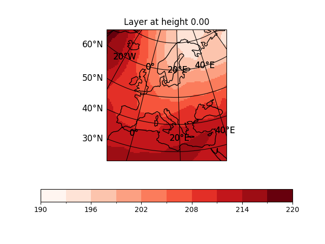
We can use the horizontal_maptransect plotter for visualizing a horizontal map transect. In this example, we use a model output of the COSMO-CLM model and display horizontal and vertical map transects.

The file T.nc is here available for download.

In [1]: import psyplot.project as psy

In [2]: temperature_ds = psy.open_dataset("data/T.nc")
   ...: temperature_ds
   ...: 
Out[2]: 
<xarray.Dataset> Size: 2MB
Dimensions:       (time: 1, level: 40, rlat: 111, rlon: 101, bnds: 2)
Coordinates:
    lat           (rlat, rlon) float32 45kB ...
    lon           (rlat, rlon) float32 45kB ...
  * rlat          (rlat) float32 444B -24.09 -23.65 -23.21 ... 23.43 23.87 24.31
  * rlon          (rlon) float32 404B -25.13 -24.69 -24.25 ... 17.99 18.43 18.87
    rotated_pole  |S1 1B ...
  * time          (time) datetime64[ns] 8B 1983-12-01T21:00:00
    time_bnds     (time, bnds) datetime64[ns] 16B ...
Dimensions without coordinates: level, bnds
Data variables:
    T             (time, level, rlat, rlon) float32 2MB ...
Attributes:
    title:           Europe 0.44 Starter Package subchain
    source:          CCLM: /work/gg0302/g266006/cclm-sp-v3.1.1/src/cclm/bin/c...
    experiment_id:   tst001
    realization:     1
    Conventions:     CF-1.4
    conventionsURL:  http://www.cfconventions.org/
    contact:         burkhardt.rockel@hzg.de
    references:      http://www.clm-community.eu/
    creation_date:   2019-06-29 18:32:13
    history:         Mon Feb  3 13:37:38 2020: ncks -v T 1983_12/out01/lffd19...
    NCO:             netCDF Operators version 4.7.5 (Homepage = http://nco.sf...

In [3]: temperature_ds.psy.plot.horizontal_maptransect(
   ...:     name="T",
   ...:     transect=0,
   ...:     cmap="Reds",
   ...:     title="Layer at height %(transect)1.2f",
   ...: )
   ...: 
Out[3]: psyplot.project.Project([    arr0: 3-dim DataArray of T, with (level, rlat, rlon)=(40, 111, 101), rotated_pole=b'', time=1983-12-01T21:00:00])

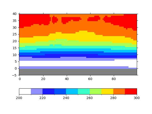
We can combine this with a vertical map transect along a given path:

In [4]: temperature_ds.psy.plot.vertical_maptransect(
   ...:     name="T",
   ...:     plot="poly",
   ...:     background="0.5",
   ...:     transform="cyl",
   ...:     xlim="minmax",
   ...: )
   ...: 
Out[4]: psyplot.project.Project([    arr1: 3-dim DataArray of T, with (level, rlat, rlon)=(40, 111, 101), rotated_pole=b'', time=1983-12-01T21:00:00])

Vertical level information

The vertical level information in such a climate model is usually given in bar. This information is not very helpful for most of the people, therefore psy-transect implements a methodology, to merge the vertical information into the data and generate a CF-conform representation of the orography. For COSMO-CLM, this information is stored in the file with the rather cryptic name lffd1980010100c.nc.

In [5]: from psy_transect import utils

In [6]: orography = psy.open_dataset("data/lffd1980010100c.nc").psy.HHL.psy[0]

In [7]: new_ds = utils.mesh_to_cf_bounds(
   ...:     orography, "level1", "level", temperature_ds
   ...: )
   ...: 

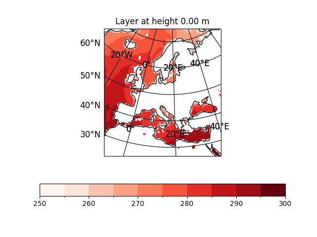
In [8]: new_ds.psy.plot.horizontal_maptransect(
   ...:     name="T",
   ...:     transect=0,
   ...:     cmap="Reds",
   ...:     title="Layer at height %(transect)1.2f m",
   ...: )
   ...: 
Out[8]: psyplot.project.Project([    arr2: 3-dim DataArray of T, with (level, rlat, rlon)=(40, 111, 101), rotated_pole=b'', time=1983-12-01T21:00:00])

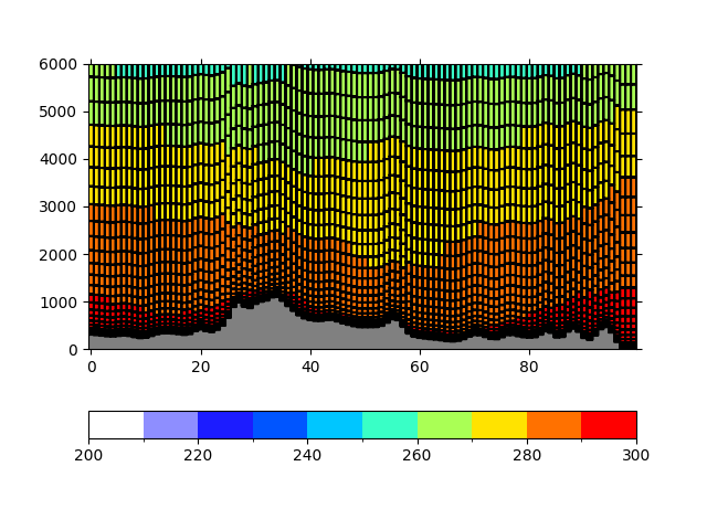
In [9]: new_ds.psy.plot.vertical_maptransect(
   ...:     name="T",
   ...:     plot="poly",
   ...:     background="0.5",
   ...:     datagrid="k-",
   ...:     transform="cyl",
   ...:     xlim="minmax",
   ...:     ylim=(0, 6000),
   ...:     yticks=np.linspace(0, 6000, 7),
   ...: )
   ...: 
Out[9]: psyplot.project.Project([    arr3: 3-dim DataArray of T, with (level, rlat, rlon)=(40, 111, 101), rotated_pole=b'', time=1983-12-01T21:00:00])

As you can see in this plot, we are able to visualize the exact orography of the model, without the need of any interpolation.

Interactive exploratory data analysis

One important aspect for transects is the interactive usage. We want to be able to connect multiple plots and visualize the vertical transect along a line that we draw. psy-transect has implemented some widgets (that we cannot demonstrate in this static documentation). You can activate it via

p1, p2 = psy.gcp(True).plotters
p1.connect_ax(p2)
p2.connect_ax(p1)