xarray Accessors

psyplot defines a DataArray and a Dataset accessor. You can use these accessors (see Xarray Internals) to visualize your data and to update your plots. The following sections will show you how to make and update plots with these accessors. The plotmethods of the accessors are the same as for the psyplot.project.plot object.

The `DatasetAccessor` dataset accessor

Importing the psyplot package registers a new dataset accessor (see xarray.register_dataset_accessor()), the DatasetAccessor. You can access it via the psy attribute of the Dataset class, i.e.

xarray.Dataset.psy

alias of DatasetAccessor

It can be used to visualize the variables in the dataset directly from the dataset itself, e.g.

In [1]: import psyplot

In [2]: ds = psyplot.open_dataset("demo.nc")

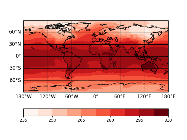
In [3]: sp = ds.psy.plot.mapplot(name="t2m", cmap="Reds")

The variable sp is a psyplot subproject of the current main project.

In [4]: print(sp)
psyplot.project.Project([    arr0: 2-dim DataArray of t2m, with (lat, lon)=(96, 192), lev=1e+05, time=1979-01-31T18:00:00])

Hence, it would be completely equivalent if you type

In [5]: import psyplot.project as psyplot

In [6]: sp = psy.plot.mapplot(ds, name="t2m", cmap="Reds")

Note that the DatasetAccessor.plot attribute has the same plotmethods as the psyplot.project.plot instance.

The `InteractiveArray` dataarray accessor

More advanced then the dataset accessor is the registered DataArray accessor, the InteractiveArray.

As well as the DatasetAccessor, it is registered as the 'psy' attribute of any DataArray, i.e.

xarray.DataArray.psy

alias of InteractiveArray

You can use it for two things:

create plots of the array
update the plots and the array

Creating plots with the dataarray accessor

Just use the plot attribute the accessor.

In [7]: import psyplot

In [8]: ds = psyplot.open_dataset("demo.nc")

In [9]: da = ds.t2m[0, 0]

# this is a two dimensional array
In [10]: print(da)
<xarray.DataArray 't2m' (lat: 96, lon: 192)> Size: 74kB
[18432 values with dtype=float32]
Coordinates:
  * lon      (lon) float64 2kB 0.0 1.875 3.75 5.625 ... 352.5 354.4 356.2 358.1
  * lat      (lat) float64 768B 88.57 86.72 84.86 83.0 ... -84.86 -86.72 -88.57
    lev      float64 8B 1e+05
    time     datetime64[ns] 8B 1979-01-31T18:00:00
Attributes:
    long_name:  Temperature
    units:      K
    code:       130
    table:      128
    grid_type:  gaussian

# and we can plot it using the mapplot plot method
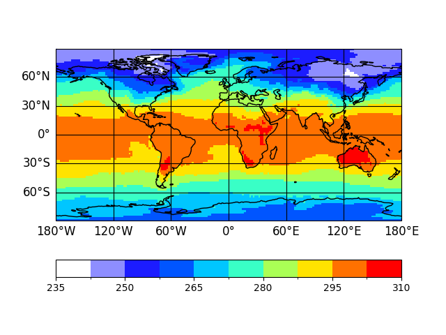
In [11]: plotter = da.psy.plot.mapplot()

The resulting plotter, an instance of the psyplot.plotter.Plotter class, is the object that visualizes the data array. It can also be accessed via the da.psy.plotter attribute. Note that the creation of such a plotter overwrites any previous plotter in the da.psy.plotter attribute.

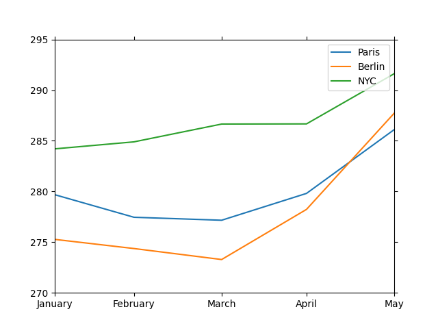
This methodology does not only work for DataArrays, but also for multiple DataArrays in a InteractiveList. This data structure is, for example, used by the psyplot.project.plot.lineplot plot method to visualize multiple lines. Consider the following example:

In [12]: ds0 = ds.isel(lev=0)  # select a subset of the dataset

# create a list of arrays at different longitudes
In [13]: l = psyplot.InteractiveList(
   ....:     [
   ....:         ds0.t2m.sel(lon=2.35, lat=48.86, method="nearest"),  # Paris
   ....:         ds0.t2m.sel(lon=13.39, lat=52.52, method="nearest"),  # Berlin
   ....:         ds0.t2m.sel(lon=-74.01, lat=40.71, method="nearest"),  # NYC
   ....:     ]
   ....: )
   ....: 

In [14]: l.arr_names = ["Paris", "Berlin", "NYC"]

# plot the list
In [15]: plotter = l.psy.plot.lineplot(xticks="data", xticklabels="%B")

Note that for the InteractiveList, the psy attribute is just the list it self. So it would have been equivalent to call

In [16]: l.plot.lineplot()

Updating plots and arrays with the dataarray accessor

The InteractiveArray accessor is designed for interactive usage of, not only the matplotlib figures, but also of the data. If you selected a subset of a dataset, e.g. via

In [17]: da = ds.t2m[0, 0]
   ....: print(da.time)  # January 1979
   ....: 
<xarray.DataArray 'time' ()> Size: 8B
array('1979-01-31T18:00:00.000000000', dtype='datetime64[ns]')
Coordinates:
    lev      float64 8B 1e+05
    time     datetime64[ns] 8B 1979-01-31T18:00:00
Attributes:
    standard_name:  time

You can change to a different slice using the InteractiveArray.update() method.

In [18]: da.psy.base = ds  # tell psyplot the source of the dataarray

In [19]: da.psy.update(time=2)
   ....: print(da.time)  # changed to March 1979
   ....: 
<xarray.DataArray 'time' ()> Size: 8B
array('1979-03-31T18:00:00.000000000', dtype='datetime64[ns]')
Coordinates:
    lev      float64 8B 1e+05
    time     datetime64[ns] 8B 1979-03-31T18:00:00
Attributes:
    standard_name:  time

The da.psy.base = ds command hereby tells the dataarray, where it is coming from, since this information is not known in the standard xarray framework.

Hint

You can avoid this, using the DatasetAccessor.create_list() method of the dataset accessor

In [20]: da = ds.psy.create_list(time=0, lev=0, name="t2m")[0]
   ....: print(da.psy.base is ds)
   ....: 
True

If you plotted the data, you can also change the formatoptions using the update() method, e.g.

# create plot

In [21]: da.psy.update(cmap="Reds")

The same holds for the Interactive list

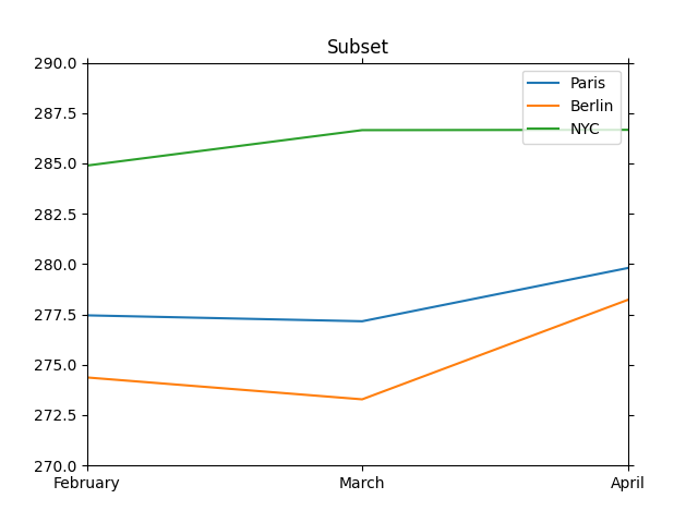
In [22]: l.update(
   ....:     time=slice(
   ....:         1, 4
   ....:     ),  # change the data by selecting a subset of the timeslice
   ....:     title="Subset",  # change a formatoption, the title of the plot
   ....: )
   ....: 