The psyplot framework

The main module we used so far, was the psyplot.project module. It is the end of a whole framework that is setup by the psyplot package.

This framework is designed in analogy to matplotlibs figure - axes - artist setup, where one figure controls multiple axes, an axes is the manager of multiple artists (e.g. a simple line) and each artist is responsible for visualizing one or more objects on the plot. The psyplot framework instead is defined through the Project - (InteractiveBase - Plotter) - Formatoption relationship.

The last to parts in this framework, the Plotter and Formatoption, are only defined through abstract base classes in this package. They are filled with contents in plugins such as the psy-simple or the psy-maps plugin (see Psyplot plugins).

The project() function

The psyplot.project.Project class (in analogy to matplotlibs Figure class) is basically a list that controls multiple plot objects. It comprises the full functionality of the package and packs it into one class, the Project class.

In analogy to pyplots figure() function, a new project can simply be created via

In [1]: import psyplot.project as psy

In [2]: p = psy.project()

This automatically sets p to be the current project which can be accessed through the gcp() method. You can also set the current project by using the scp() function.

Note

We highly recommend to use the project() function to create new projects instead of creating projects from the Project. This ensures the right numbering of the projects of old projects.

The project uses the plotters from the psyplot.plotter module to visualize your data. Hence you can add new plots and new data to the project by using the Project.plot attribute or the psyplot.project.plot attribute which targets the current project. The return types of the plotting methods are again instances of the Project class, however we consider them as subprojects in contrast main projects that are created through the project() function. There is basically no difference but the result of the Project.is_main attribute which is False for subprojects. Hence, each new plot creates a subproject but also stores the data array in the corresponding main project of the Project instance from which the plot method has been called. The newly created subproject can be accessed via

In [3]: sp = psy.gcp()

whereas the current main project can be accessed via

In [4]: p = psy.gcp(main=True)

Plots created by a specific method of the Project.plot attribute may however be accessed via the corresponding attribute of the Project class. The following example creates three subprojects, two with the mapplot and mapvector methods from the psy-maps plugin and one with the simple lineplot method from the psy-simple plugin to visualize simple lines.

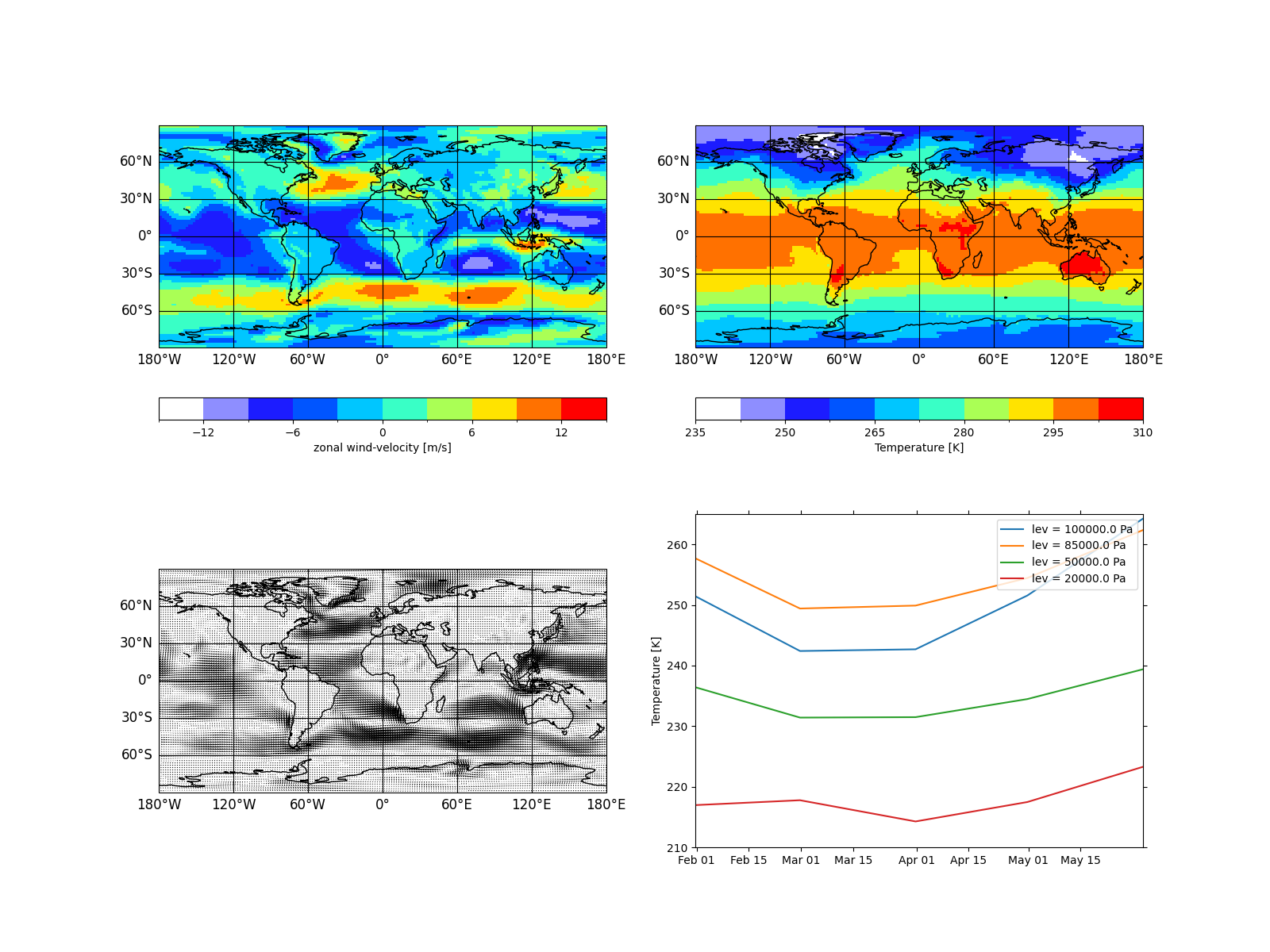
In [5]: import matplotlib.pyplot as plt

In [6]: import cartopy.crs as ccrs

# the subplots for the maps (need cartopy projections)
In [7]: ax = list(psy.multiple_subplots(2, 2, n=3, for_maps=True))

# the subplot for the line plot
In [8]: ax.append(plt.gcf().add_subplot(2, 2, 4))

# scalar field of the zonal wind velocity in the file demo.nc
In [9]: psy.plot.mapplot('demo.nc', name='u', ax=ax[0], clabel='{desc}')
Out[9]: psyplot.project.Project([    arr0: 2-dim DataArray of u, with (lat, lon)=(96, 192), lev=1e+05, time=1979-01-31T18:00:00])

# a second scalar field of temperature
In [10]: psy.plot.mapplot('demo.nc', name='t2m', ax=ax[1], clabel='{desc}')
Out[10]: psyplot.project.Project([    arr1: 2-dim DataArray of t2m, with (lat, lon)=(96, 192), lev=1e+05, time=1979-01-31T18:00:00])

# a vector plot projected on the earth
In [11]: psy.plot.mapvector('demo.nc', name=[['u', 'v']], ax=ax[2],
   ....:                    attrs={'long_name': 'Wind speed'})
   ....: 
Out[11]: psyplot.project.Project([    arr2: 3-dim DataArray of u, v, with (variable, lat, lon)=(2, 96, 192), lev=1e+05, time=1979-01-31T18:00:00])

In [12]: psy.plot.lineplot('demo.nc', name='t2m', x=0, y=0, z=range(4),
   ....:                   ax=ax[3], xticklabels='%b %d', ylabel='{desc}',
   ....:                   legendlabels='%(zname)s = %(z)s %(zunits)s')
   ....: 
Out[12]: 
psyplot.project.Project([arr3: psyplot.data.InteractiveList([
    arr0: 1-dim DataArray of t2m, with (time)=(5,), lon=0.0, lat=88.57, lev=1e+05,
    arr1: 1-dim DataArray of t2m, with (time)=(5,), lon=0.0, lat=88.57, lev=8.5e+04,
    arr2: 1-dim DataArray of t2m, with (time)=(5,), lon=0.0, lat=88.57, lev=5e+04,
    arr3: 1-dim DataArray of t2m, with (time)=(5,), lon=0.0, lat=88.57, lev=2e+04])])

The latter is now the current subproject we could access via psy.gcp(). However we can access all of them through the main project

In [13]: mp = psy.gcp(True)

In [14]: mp  # all arrays
Out[14]: 
2 Main psyplot.project.Project([
    arr0: 2-dim DataArray of u, with (lat, lon)=(96, 192), lev=1e+05, time=1979-01-31T18:00:00,
    arr1: 2-dim DataArray of t2m, with (lat, lon)=(96, 192), lev=1e+05, time=1979-01-31T18:00:00,
    arr2: 3-dim DataArray of u, v, with (variable, lat, lon)=(2, 96, 192), lev=1e+05, time=1979-01-31T18:00:00,
    arr3: psyplot.data.InteractiveList([
        arr0: 1-dim DataArray of t2m, with (time)=(5,), lon=0.0, lat=88.57, lev=1e+05,
        arr1: 1-dim DataArray of t2m, with (time)=(5,), lon=0.0, lat=88.57, lev=8.5e+04,
        arr2: 1-dim DataArray of t2m, with (time)=(5,), lon=0.0, lat=88.57, lev=5e+04,
        arr3: 1-dim DataArray of t2m, with (time)=(5,), lon=0.0, lat=88.57, lev=2e+04])])

In [15]: mp.mapplot  # all scalar fields
Out[15]: 
psyplot.project.Project([
    arr0: 2-dim DataArray of u, with (lat, lon)=(96, 192), lev=1e+05, time=1979-01-31T18:00:00,
    arr1: 2-dim DataArray of t2m, with (lat, lon)=(96, 192), lev=1e+05, time=1979-01-31T18:00:00])

In [16]: mp.mapvector  # all vector plots
Out[16]: psyplot.project.Project([    arr2: 3-dim DataArray of u, v, with (variable, lat, lon)=(2, 96, 192), lev=1e+05, time=1979-01-31T18:00:00])

In [17]: mp.maps  # all data arrays that are plotted on a map
Out[17]: 
psyplot.project.Project([
    arr0: 2-dim DataArray of u, with (lat, lon)=(96, 192), lev=1e+05, time=1979-01-31T18:00:00,
    arr1: 2-dim DataArray of t2m, with (lat, lon)=(96, 192), lev=1e+05, time=1979-01-31T18:00:00,
    arr2: 3-dim DataArray of u, v, with (variable, lat, lon)=(2, 96, 192), lev=1e+05, time=1979-01-31T18:00:00])

In [18]: mp.lineplot # the simple plot we created
Out[18]: 
psyplot.project.Project([arr3: psyplot.data.InteractiveList([
    arr0: 1-dim DataArray of t2m, with (time)=(5,), lon=0.0, lat=88.57, lev=1e+05,
    arr1: 1-dim DataArray of t2m, with (time)=(5,), lon=0.0, lat=88.57, lev=8.5e+04,
    arr2: 1-dim DataArray of t2m, with (time)=(5,), lon=0.0, lat=88.57, lev=5e+04,
    arr3: 1-dim DataArray of t2m, with (time)=(5,), lon=0.0, lat=88.57, lev=2e+04])])

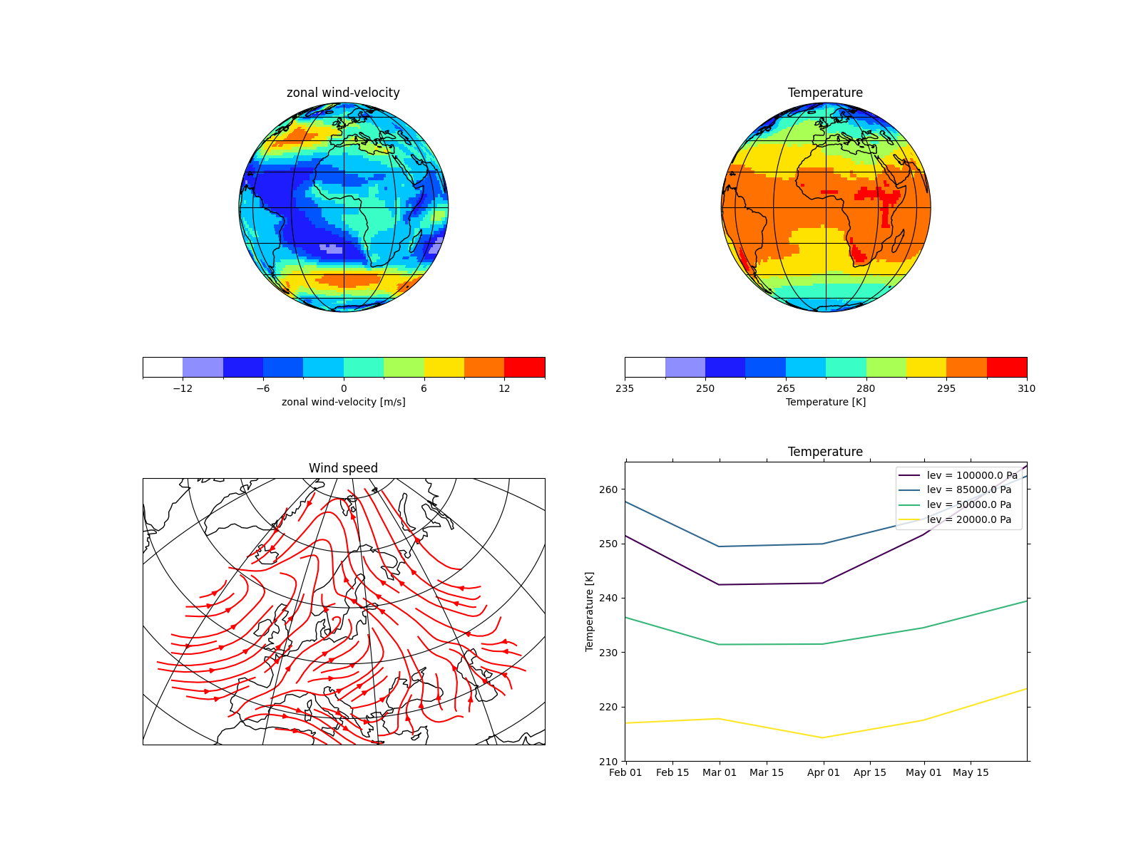
The advantage is, since every plotter has different formatoptions, we can now update them very easily. For example lets update the arrowsize to 1 (which only works for the mapvector plots), the projection to an orthogonal (which only works for maps), the simple plots to use the 'viridis' colormap for color coding the lines and for all we choose their title corresponding to the variable names

In [19]: p.maps.update(projection='ortho')

In [20]: p.mapvector.update(color='r', plot='stream', lonlatbox='Europe')

In [21]: p.lineplot.update(color='viridis')

In [22]: p.update(title='%(long_name)s')

The InteractiveBase and the Plotter classes

Interactive data objects

The next level are instances of the InteractiveBase class. This abstract base class provides an interface between the data and the visualization. Hence a plotter (that’s how we call instances of the Plotter class) will deal with the subclasses of the InteractiveBase:

InteractiveArray(xarray_obj, *args, **kwargs)	Interactive psyplot accessor for the data array
InteractiveList(*args, **kwargs)	List of InteractiveArray instances that can be plotted itself

Those classes (in particular the InteractiveArray) keep the reference to the base dataset to allow the update of the dataslice you are plotting. The InteractiveList class can be used in a plotter for the visualization of multiple InteractiveArray instances (see for example the psyplot.plotter.simple.LinePlotter and psyplot.plotter.maps.CombinedPlotter classes). Furthermore those data instances have a plotter attribute that is usually occupied by an instance of a Plotter subclass.

Note

The InteractiveArray serves as a DataArray accessor. After you imported psyplot, you can access it via the psy attribute of a DataArray, i.e. via

In [23]: import xarray as xr

In [24]: xr.DataArray([]).psy
Out[24]: <psyplot.data.InteractiveArray at 0x7fb845d23610>

Visualization objects

Each plotter class is the coordinator of several visualization options. Thereby the Plotter class itself contains only the structural functionality for managing the formatoptions that do the real work. The plotters for the real usage are defined in plugins like the psy-simple or the psy-maps package.

Hence each InteractiveBase instance is visualized by exactly one Plotter class. If you don’t want to use the project framework, the initialization of such an instance nevertheless straight forward. Just open a dataset, extract the right data array and plot it

In [25]: from psyplot import open_dataset

In [26]: from psy_maps.plotters import FieldPlotter

In [27]: ds = open_dataset('demo.nc')

In [28]: arr = ds.t2m[0, 0]

In [29]: plotter = FieldPlotter(arr)

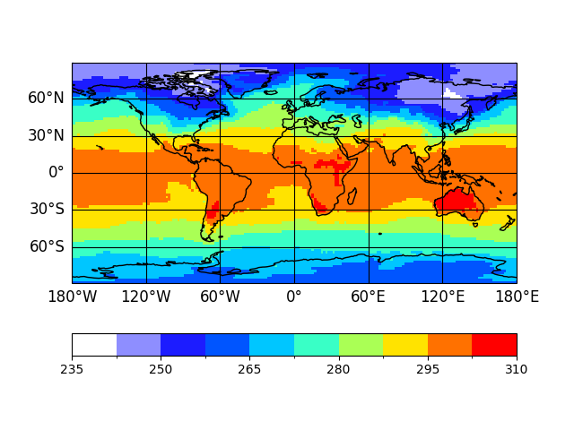
Now we created a plotter with all it’s formatoptions:

In [30]: type(plotter), plotter
Out[30]: 
(psy_maps.plotters.FieldPlotter,
 {'levels': None,
  'interp_bounds': None,
  'plot': 'mesh',
  'miss_color': None,
  'background': 'rc',
  'transpose': False,
  'projection': 'cf',
  'transform': 'cf',
  'clon': None,
  'clat': None,
  'lonlatbox': None,
  'lsm': {'res': '110m', 'linewidth': 1.0, 'coast': 'k'},
  'stock_img': False,
  'grid_color': 'k',
  'grid_labels': None,
  'grid_labelsize': 12.0,
  'grid_settings': {},
  'xgrid': True,
  'ygrid': True,
  'map_extent': None,
  'google_map_detail': None,
  'datagrid': None,
  'clip': None,
  'cmap': 'white_blue_red',
  'bounds': [<BoundsMethod.rounded: 'rounded'>, None, 0.0, 100.0, None, None],
  'extend': 'neither',
  'cbar': {'b'},
  'clabel': '',
  'clabelsize': 'medium',
  'clabelweight': None,
  'cbarspacing': 'uniform',
  'clabelprops': {},
  'cticks': None,
  'cticklabels': None,
  'cticksize': 'medium',
  'ctickweight': None,
  'ctickprops': {},
  'mask_datagrid': True,
  'tight': False,
  'maskless': None,
  'maskleq': None,
  'maskgreater': None,
  'maskgeq': None,
  'maskbetween': None,
  'mask': None,
  'title': '',
  'titlesize': 'large',
  'titleweight': None,
  'titleprops': {},
  'figtitle': '',
  'figtitlesize': 12.0,
  'figtitleweight': None,
  'figtitleprops': {},
  'text': [],
  'post_timing': 'never',
  'post': None})

You can use the show_keys(), show_summaries() and show_docs() methods to have a look into the documentation into the formatoptions or you simply use the builtin help() function for it:

>>> help(plotter.clabel)

The update methods are the same as for the Project class. You can use the psyplot.data.InteractiveArray.update() via arr.psy.update() which updates the data and forwards the formatoptions to the Plotter.update() method.

Note

Plotters are subclasses of dictionaries where each item represents the key-value pair of one formatoption. Anyway, although you could now simply set a formatoption like you set an item for a dictionary via

In [31]: plotter['clabel'] = 'my label'

or equivalently

In [32]: plotter.clabel = 'my label'

this would not change the plot! Instead you have to use the psyplot.plotter.Plotter.update() method, i.e.

In [33]: plotter.update(clabel='my label')

Formatoptions

Formatoptions are the core of the visualization in the psyplot framework. They conceptually correspond to the basic matplotlib.artist.Artist and inherit from the abstract Formatoption class. Each plotter is set up through it’s formatoptions where each formatoption has a unique formatoption key inside the plotter. This formatoption key (e.g. ‘title’ or ‘clabel’) is what is used for updating the plot etc. You can find more information in How to implement your own plotters and plugins .