Note
This example requires the demo.nc file.
Applying your own post processing
This demo shows you how to use the post formatoption to apply your own post processing scripts.
It requires the 'demo.nc' netCDF file, netCDF4 and the psy-maps plugin.
[1]:
import psyplot.project as psy
%matplotlib inline
%config InlineBackend.close_figures = False
Usage
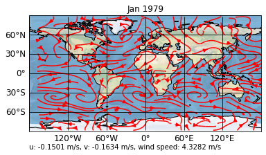
The post formatoption let’s you apply your own script to modify your data. Let’s start with a simple plot of the wind speed:
[2]:
sp = psy.plot.mapvector('demo.nc', name=[['u', 'v']], plot='stream',
                        color='red', title='%b %Y')
print(sp)
psyplot.project.Project([ arr0: 3-dim DataArray of u, v, with (variable, lat, lon)=(2, 96, 192), lev=1e+05, time=1979-01-31T18:00:00])

It is hard to see the continents below this amount of arrows. So we might want to enhance our plot with cartopy’s stock_img.
But since there is now formatoption for it, we can now either define a new plotter and add the formatoption, or we use the post formatoption.
[3]:
sp.update(enable_post=True,
          post='self.stock_img = self.ax.stock_img()')
sp.show()

The first parameter enable_post=True sets the enable_post attribute of the plotter to True. This attribute is by default set to False because it is always a security vulnerability to use the built-in exec function which is used by the post formatoption. We could, however, already have included this in our first definition of the project via
sp = psy.plot.mapvector('demo.nc', name=[['u', 'v']], plot='stream', color='red',
                        enable_post=True)
The second parameter post='self.ax.stock_img()' updates the post formatoption. It accepts an executable python script as a string. Note that we make use of the self variable, the only variable that is given to the script. It is the Formatoption instance that performs the update. Hence you can access all the necessary attributes and informations:
the axes through
self.axthe figure through
self.ax.figurethe data that is plotted through
self.datathe raw data from the dataset through
self.raw_datathe plotter through
self.plotterany other formatoption in the plotter, e.g. the
titlethroughself.plotter.title
For example, let’s add another feature that adds the mean of the plotted variables to the plot. For this, let’s first have a look into the plot_data attribute of the plotter which includes the data that is visualized and that is accessible through the data attribute of the post formatoption:
[4]:
sp.plotters[0].plot_data
[4]:
<xarray.DataArray (variable: 2, lat: 96, lon: 192)>
array([[[-5.548854  , -5.470729  , -5.3847914 , ..., -5.7344007 ,
         -5.6802015 , -5.618678  ],
        [-4.1748304 , -4.246608  , -4.30276   , ..., -3.8872328 ,
         -3.9927015 , -4.0898695 ],
        [-2.2866468 , -2.6035414 , -2.8896742 , ..., -1.2148695 ,
         -1.585475  , -1.94485   ],
        ...,
        [-1.9463148 , -1.8501234 , -1.7676039 , ..., -2.3105726 ,
         -2.1772718 , -2.0556898 ],
        [-2.6640882 , -2.547389  , -2.434596  , ..., -3.0415297 ,
         -2.9111586 , -2.785182  ],
        [-3.4873304 , -3.3711195 , -3.2514906 , ..., -3.8120375 ,
         -3.7080336 , -3.5996351 ]],

       [[ 2.3220043 ,  2.5290356 ,  2.7336254 , ...,  1.6891918 ,
          1.9015942 ,  2.1125317 ],
        [ 1.3434887 ,  1.6203442 ,  1.906477  , ...,  0.57639885,
          0.8200512 ,  1.0759106 ],
        [ 0.1662426 ,  0.6325512 ,  1.1335278 , ..., -0.97780037,
         -0.64235115, -0.26002693],
        ...,
        [-2.2136402 , -2.2927418 , -2.3772144 , ..., -1.996355  ,
         -2.0661793 , -2.138445  ],
        [-2.2043629 , -2.2819996 , -2.3586597 , ..., -1.9577808 ,
         -2.04323   , -2.1252613 ],
        [-1.8645191 , -1.9768238 , -2.0837574 , ..., -1.4978199 ,
         -1.624773  , -1.7468433 ]]], dtype=float32)
Coordinates:
  * lon       (lon) float64 0.0 1.875 3.75 5.625 7.5 ... 352.5 354.4 356.2 358.1
  * lat       (lat) float64 88.57 86.72 84.86 83.0 ... -84.86 -86.72 -88.57
    lev       float64 1e+05
    time      datetime64[ns] 1979-01-31T18:00:00
  * variable  (variable) <U1 'u' 'v'
Attributes:
    CDI:          Climate Data Interface version 1.6.8 (http://mpimet.mpg.de/...
    Conventions:  CF-1.4
    history:      Mon Aug 17 22:51:40 2015: cdo -r copy test-t2m-u-v.nc test-...
    title:        Test file
    CDO:          Climate Data Operators version 1.6.8rc2 (http://mpimet.mpg....
    long_name:    zonal wind-velocity
    units:        m/s
    code:         131
    table:        128
grid_type: gaussianIt is a 3-dimensional array, where the first dimension consists of the zonal wind speed 'u' and the meridional wind speed 'v'. So let’s add their means as a text to the plot:
[5]:
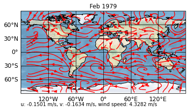
sp.update(post="""
self.stock_img = self.ax.stock_img()
umean = self.data[0].mean().values
vmean = self.data[1].mean().values
abs_mean = ((self.data[0]**2 + self.data[1]**2)**0.5).mean().values
self.text = self.ax.text(
    0., -0.15,
    'u: %1.4f m/s, v: %1.4f m/s, wind speed: %1.4f m/s' % (
        umean, vmean, abs_mean),
    transform=self.ax.transAxes)""")
sp.show()
Timing
psyplot is intended to work interactively. By default, the post formatoption is only updated when you personally update it. However, you can modify this timing using the post_timing formatoption. It can be either
'never': The default which requires a manual update'replot': To update it when the data changes'always': To always update it.
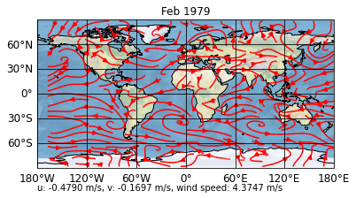
For example, in the current setting, when we change the data to the second time step via
[6]:
sp.update(time=1)
print(sp)
sp.show()
psyplot.project.Project([ arr0: 3-dim DataArray of u, v, with (variable, lat, lon)=(2, 96, 192), lev=1e+05, time=1979-02-28T18:00:00])
Our means are not updated, for this, we have to
set the
post_timingto'replot'slightly modify our
postscript to not plot two texts above each other
[7]:
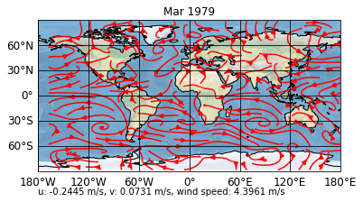
sp.update(post_timing='replot', post="""
self.stock_img = self.ax.stock_img()
umean = self.data[0].mean().values
vmean = self.data[1].mean().values
abs_mean = ((self.data[0]**2 + self.data[1]**2)**0.5).mean().values
if hasattr(self, 'text'):
    text = self.text
else:
    text = self.ax.text(0., -0.15, '',
                        transform=self.ax.transAxes)
text.set_text(
    'u: %1.4f m/s, v: %1.4f m/s, wind speed: %1.4f m/s' % (
        umean, vmean, abs_mean))""")
sp.show()
Now, if we update to the third timestep, our means are also calculated
[8]:
sp.update(time=2)
sp.show()
Saving and loading
Saving a project is straight forward via the save_project method
[9]:
d = sp.save_project()
However, when loading the project, the enable_post attribute is (for security reasons) again set to False. So if you are sure you can trust the post processing scripts in the post formatoption, load your project with enable_post=True
[10]:
psy.close('all')
sp = psy.Project.load_project(d, enable_post=True)

[11]:
psy.close('all')