Interactive online version:
Note
Creating and accessing a fit
This example shows you, how you can easily calculate and visualize a fit to your data
[1]:
import numpy as np
import xarray as xr
import psyplot.project as psy
%matplotlib inline
%config InlineBackend.close_figures = False
First we start with some example data to make a linear regression from the equation y(x) = 4 * x + 30
[2]:
x = np.linspace(0, 100)
y = x * 4 + 30 + 50* np.random.normal(size=x.size)
ds = xr.Dataset({'x': xr.Variable(('experiment', ), x),
                 'y': xr.Variable(('experiment', ), y)})
ds
[2]:
<xarray.Dataset>
Dimensions:  (experiment: 50)
Dimensions without coordinates: experiment
Data variables:
    x        (experiment) float64 0.0 2.041 4.082 6.122 ... 95.92 97.96 100.0
y (experiment) float64 61.33 -7.603 6.917 138.6 ... 442.7 406.0 457.9We can show this input data using the lineplot plot method from the psy-simple plugin:
[3]:
raw = psy.plot.lineplot(
    ds, name='y', coord='x', linewidth=0, marker='o', legendlabels='raw data',
    legend='upper left')
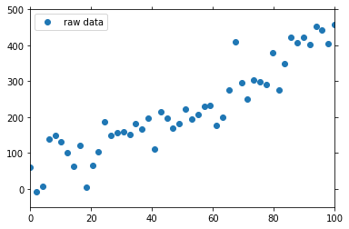
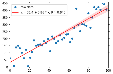
The visualization of the fit is straight forward using the linreg plot method:
[4]:
fit = psy.plot.linreg(ds, ax=raw.plotters[0].ax, name='y', coord='x',
                      legendlabels='fit', color='red')
fit.share(raw[0], keys='legend')
fit.show()
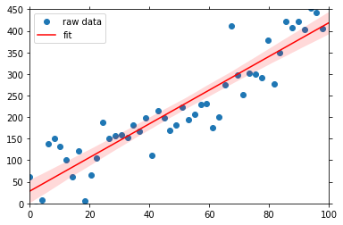
The shaded red area displays the 95% confidence interval. To access the data for the fit, just use the plot_data attribute:
[5]:
data = fit[0].psy.plotter.plot_data
data[0]
[5]:
<xarray.DataArray 'y' (variable: 3, x: 100)>
array([[2.84468219e+01, 3.23881507e+01, 3.63294794e+01, 4.02708081e+01,
4.42121369e+01, 4.81534656e+01, 5.20947943e+01, 5.60361231e+01,
5.99774518e+01, 6.39187805e+01, 6.78601093e+01, 7.18014380e+01,
7.57427667e+01, 7.96840955e+01, 8.36254242e+01, 8.75667529e+01,
9.15080817e+01, 9.54494104e+01, 9.93907391e+01, 1.03332068e+02,
1.07273397e+02, 1.11214725e+02, 1.15156054e+02, 1.19097383e+02,
1.23038712e+02, 1.26980040e+02, 1.30921369e+02, 1.34862698e+02,
1.38804026e+02, 1.42745355e+02, 1.46686684e+02, 1.50628013e+02,
1.54569341e+02, 1.58510670e+02, 1.62451999e+02, 1.66393328e+02,
1.70334656e+02, 1.74275985e+02, 1.78217314e+02, 1.82158643e+02,
1.86099971e+02, 1.90041300e+02, 1.93982629e+02, 1.97923957e+02,
2.01865286e+02, 2.05806615e+02, 2.09747944e+02, 2.13689272e+02,
2.17630601e+02, 2.21571930e+02, 2.25513259e+02, 2.29454587e+02,
2.33395916e+02, 2.37337245e+02, 2.41278574e+02, 2.45219902e+02,
2.49161231e+02, 2.53102560e+02, 2.57043889e+02, 2.60985217e+02,
2.64926546e+02, 2.68867875e+02, 2.72809203e+02, 2.76750532e+02,
2.80691861e+02, 2.84633190e+02, 2.88574518e+02, 2.92515847e+02,
2.96457176e+02, 3.00398505e+02, 3.04339833e+02, 3.08281162e+02,
3.12222491e+02, 3.16163820e+02, 3.20105148e+02, 3.24046477e+02,
3.27987806e+02, 3.31929134e+02, 3.35870463e+02, 3.39811792e+02,
...
1.25324912e+02, 1.28903319e+02, 1.32668913e+02, 1.36404229e+02,
1.39988881e+02, 1.43645655e+02, 1.47293475e+02, 1.50808874e+02,
1.54553191e+02, 1.58425617e+02, 1.62189376e+02, 1.65790721e+02,
1.69615244e+02, 1.73351043e+02, 1.77072920e+02, 1.80835091e+02,
1.84798150e+02, 1.88753512e+02, 1.92464612e+02, 1.96255140e+02,
2.00196228e+02, 2.04303311e+02, 2.08195595e+02, 2.11918082e+02,
2.15556040e+02, 2.19369405e+02, 2.23100396e+02, 2.26814236e+02,
2.30575589e+02, 2.34316916e+02, 2.38065564e+02, 2.41759006e+02,
2.45630446e+02, 2.49801704e+02, 2.53749253e+02, 2.57799191e+02,
2.61946752e+02, 2.66134904e+02, 2.70318870e+02, 2.74404279e+02,
2.78297886e+02, 2.82153962e+02, 2.86196926e+02, 2.90150172e+02,
2.94102695e+02, 2.98053418e+02, 3.02004141e+02, 3.05954864e+02,
3.10265777e+02, 3.14645738e+02, 3.18939866e+02, 3.23194135e+02,
3.27389216e+02, 3.31671252e+02, 3.35827378e+02, 3.40135908e+02,
3.44478408e+02, 3.48838601e+02, 3.53061501e+02, 3.57368418e+02,
3.61676792e+02, 3.65986328e+02, 3.70295623e+02, 3.74687628e+02,
3.78996209e+02, 3.83253531e+02, 3.87529746e+02, 3.91836240e+02,
3.96024396e+02, 4.00453434e+02, 4.04843322e+02, 4.09072400e+02,
4.13380930e+02, 4.17689461e+02, 4.21996439e+02, 4.26137269e+02,
4.30539943e+02, 4.34745627e+02, 4.39089335e+02, 4.43420969e+02]])
Coordinates:
* x (x) float64 0.0 1.01 2.02 3.03 4.04 ... 96.97 97.98 98.99 100.0
* variable (variable) <U7 'y' 'min_err' 'max_err'
Attributes:
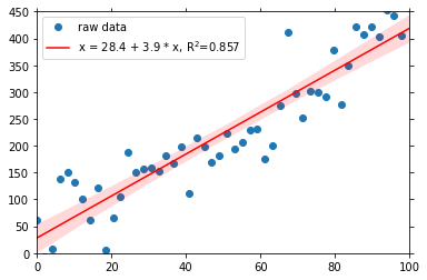
slope: 3.9019154467129207
intercept: 28.446821926887775
rsquared: 0.8571328207787087You see, that there are new attributes, rsquared, intercept and slope, the characteristics of the fit. As always with the dataset attributes in psyplot, you can visualize them, for example in the legend:
[6]:
fit.update(legendlabels='%(yname)s = %(intercept).3g + %(slope).3g * %(xname)s, R$^2$=%(rsquared).3g')
fit.show()
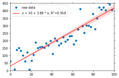
To improve the fit, we can also force the line to go through a given fix point. For example here, we know, that the fit crosses the y-line at 30:
[7]:
fit.update(fix=30)
fit.show()
That works for any other point as well. E.g. we also know, that the line goes through y = 4 * 10 + 30 = 70:
[8]:
fit.update(fix=[(10, 70)])
fit.show()
For more informations, look into the formatoptions of the regression group
[9]:
fit.summaries('regression')
xrange
    Specify the range for the fit to use for the x-dimension
yrange
    Specify the range for the fit to use for the y-dimension
line_xlim
    Specify how wide the range for the plot should be
p0
    Initial parameters for the :func:`scipy.optimize.curve_fit` function
fit
    Choose the linear fitting method
fix
    Force the fit to go through a given point
nboot
    Set the number of bootstrap resamples for the confidence interval
ci
    Draw a confidence interval
ideal
    Draw an ideal line of the fit
[10]:
psy.close('all')