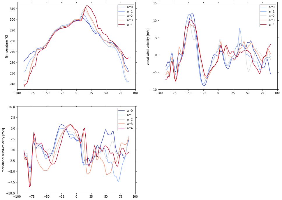
Line plot demo

This example shows you how to make a line plot using the psyplot.project.ProjectPlotter.lineplot method.

[1]:

import psyplot.project as psy
import numpy as np
%config InlineBackend.close_figures = False

[2]:

axes = iter(psy.multiple_subplots(2, 2, n=3))
for var in ['t2m', 'u', 'v']:
    psy.plot.lineplot(
        'demo.nc',  # netCDF file storing the data
        name=var, # one plot for each variable
        t=range(5),  # one line for each time step
        z=0, x=0,      # choose latitude and longitude as dimensions
        ylabel="{desc}",  # use the longname and units on the y-axis
        ax=next(axes),
        color='coolwarm',
    )

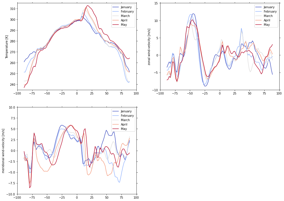
Okay, now we want to show the legend. As we show one line per timestep (and actually it’s one line per month), we might want to label the lines accordingly. The legendlabels formatoption can be automatically used for this, and we can use pythons built-in datetime formatting to format the time.

[3]:

sp = psy.gcp(True)
sp.update(
    legendlabels="%B",   # use the Month as label for the legend
)
sp.show()

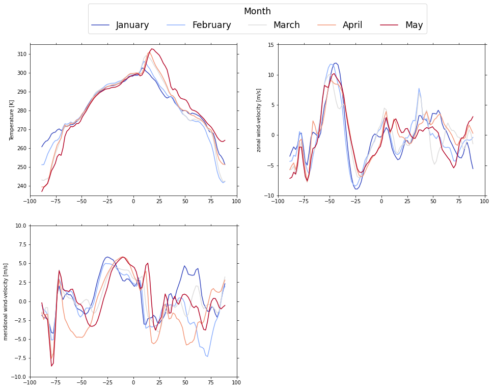
The legend is the same for all plots, so let’s disable it for the last two, and show it for the first one above the plots. We can use the legend formatoption for this, that accepts a boolean (to enable or disable the legend), or a dictionary with keyword arguments for matplotlibs legend function.

[4]:

sp[1:].update(legend=False)  # disable the legend for the second and third plot
sp[0].psy.update(
    legend=dict(
        title="Month",
        loc="upper center",
        bbox_to_anchor=(1.1, 1.3),
        ncol=5,
        fontsize="xx-large",
        title_fontsize="xx-large",
    )
)
sp.show()

[5]:

sp.close()

Visualizing uncertainties

The lineplot plotmethod also supports the visualization of uncertainty intervals. For this example, let’s assume the horizontal windspeed u has an uncertainty of 3 meter per second.

We save this constant variable in our dataset as u_std

[6]:

ds = psy.open_dataset("demo.nc")
ds["u_std"] = ds.u.copy(data=np.ones_like(ds.u) * 3)
ds

To visualize this uncertainty, we need to pass it as name=[[["u", "u_std"]]] to the lineplot method.

[7]:

sp = ds.psy.plot.lineplot(
    name=[[["u", "u_std"]]],
    t=range(2),          # one line for each time step
    z=0, x=0,            # choose latitude and longitude as dimensions
    ylabel="{desc}",     # use the longname and units on the y-axis
    xlabel="{desc}",     # use the longname and units on the x-axis
    color="coolwarm",
    legendlabels="%B",   # use the Month as label for the legend ()
    legend={"loc": "upper center", "bbox_to_anchor": (0.5, 1.2), "ncol": 2, "title": "Month"},
)

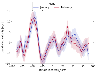
This structure parameters for name is important here, because it tells the lineplot how to structure the data. Using this syntax, our project sp now holds a list two 2D arrays, one for each line.

[8]:

sp

[8]:

psyplot.project.Project([arr3: psyplot.data.InteractiveList([
    arr0: 2-dim DataArray of u, u_std, with (variable, lat)=(2, 96), lon=0.0, lev=1e+05, time=1979-01-31T18:00:00,
    arr1: 2-dim DataArray of u, u_std, with (variable, lat)=(2, 96), lon=0.0, lev=1e+05, time=1979-02-28T18:00:00])])

Using name=[[["u", "u_std"]]] is effectively the same as using ds[["u", "u_std"]].to_array().

[9]:

sp[0][0]

[10]:

ds[["u", "u_std"]].isel(time=0, lon=0, lev=0).to_array()

[11]:

psy.close('all')