This page was generated from maps/example_ugrid.ipynb.
Interactive online version:

Note

This examples needs the following files:

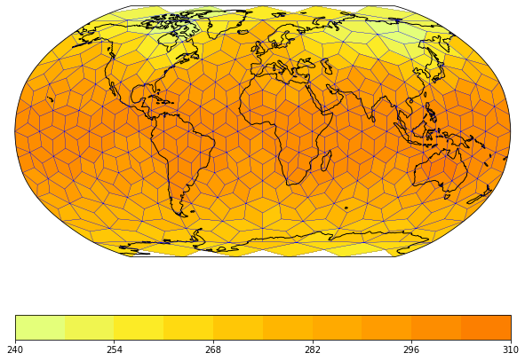
Visualizing unstructured data

Example visualization of unstructured ICON and UGRID data.

Here we show, how the psy-maps plugin can visualize the unstructured grid of the Earth System Model ICON from the Max-Planck-Institute for Meteorology in Hamburg, Germany, and data following the unstructured grids (UGRID). The visualization works the same as for normal rectilinear grids. Internally, however, the coordinates are interpreted in a completely different way (see below for a detailed explanation).

[1]:

import psyplot.project as psy
import matplotlib as mpl
%matplotlib inline
%config InlineBackend.close_figures = False

[2]:

psy.rcParams['plotter.maps.xgrid'] = False
psy.rcParams['plotter.maps.ygrid'] = False
mpl.rcParams['figure.figsize'] = [10., 8.]

Visualizing UGRID data

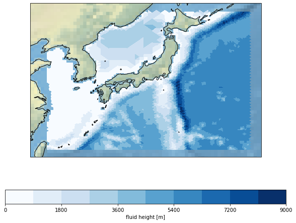
A widely accepted approach for unstructured grids are the so-called UGRID Conventions. For a demonstration, we use the 'ugrid_demo.nc' netCDF file that contains sea surface height of a Tsunami simulation. We use the load parameter, to directly load it into memory. That speeds up the plotting of the data.

psyplot automatically recognizes the UGRID conventions and adapts it’s plotting algorithm for displaying the data. For this simulation, let’s focus on Japan. We use the maskleq keyword here to mask the land surface and display a stock_img on the continents.

[3]:

tsunami = psy.plot.mapplot(
    'ugrid_demo.nc', name='Mesh2_height', load=True,
    maskleq=0, lonlatbox='Japan', cmap='Blues',
    clabel='{desc}', stock_img=True, lsm='50m')

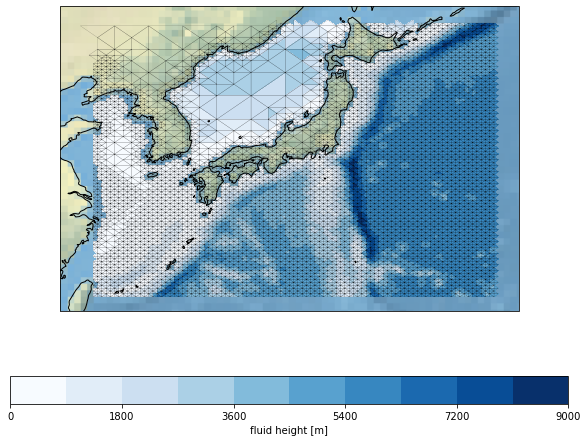
To visualize the unstructured grid, we can use the datagrid formatoption. It excepts a string or the line properties.

[4]:

tsunami.docs('datagrid')

datagrid
========
Show the grid of the data

This formatoption shows the grid of the data (without labels)

Possible types
--------------
None
    Don't show the data grid
str
    A linestyle in the form ``'k-'``, where ``'k'`` is the color and
    ``'-'`` the linestyle.
dict
    any keyword arguments that are passed to the plotting function (
    :func:`matplotlib.pyplot.triplot` for unstructured grids and
    :func:`matplotlib.pyplot.hlines` for rectilinear grids)

See Also
--------
mask_datagrid: To display cells with NaN
See Also
--------
xgrid
ygrid

[5]:

tsunami.update(datagrid={'c': 'k', 'lw': 0.1})
tsunami.show()

[6]:

tsunami.close()

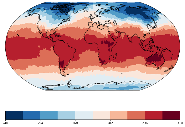
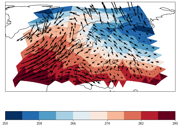
Visualizing scalar and vector ICON data

This section requires the psy-maps plugin and the file 'icon_grid_demo.nc' which contains one variable for the temperature, one for zonal and one for the meridional wind direction.

The visualization works the same way as for a usual rectangular grid. We choose a robinson projection and a colormap ranging from blue to red.

[7]:

maps = psy.plot.mapplot('icon_grid_demo.nc', name='t2m', projection='robin',
                        cmap='RdBu_r')

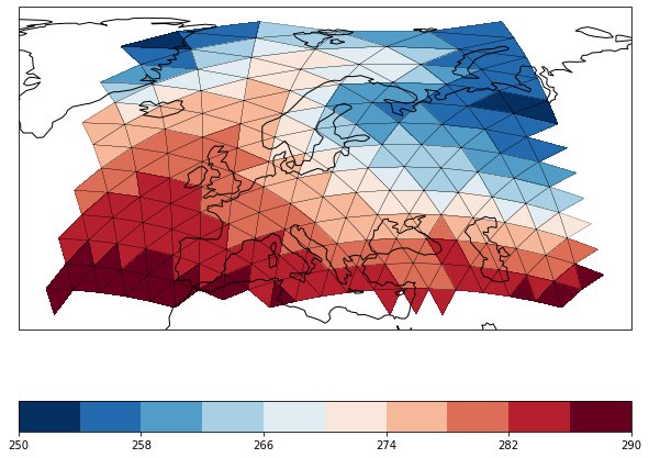
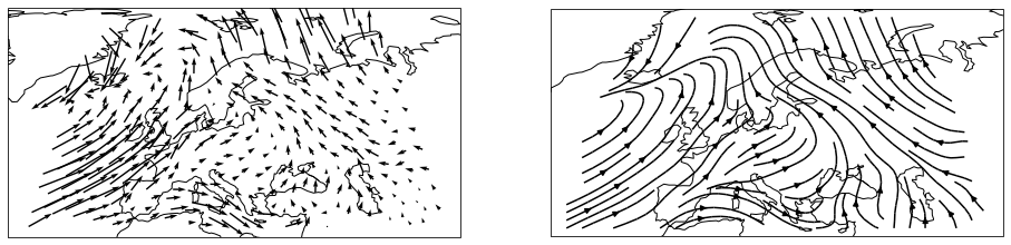
We can again zoom in to Europe and use the datagrid formatoption to display the triangular grid.

[8]:

maps.update(lonlatbox='Europe', datagrid=dict(color='k', linewidth=0.2))
maps.show()

The same works for vector data

[9]:

vectors = psy.plot.mapvector(
    'icon_grid_demo.nc', name=[['u', 'v']] * 2, projection='robin',
    ax=(1, 2), lonlatbox='Europe')
vectors.plotters[0].update(arrowsize=100)
vectors.plotters[1].update(plot='stream')

And combined scalar and vector fields

[10]:

combined = psy.plot.mapcombined(
    'icon_grid_demo.nc', name=[['t2m', ['u', 'v']]], projection='robin',
    lonlatbox='Europe', arrowsize=100, cmap='RdBu_r', datagrid={'c': 'k', 'lw': 0.1})

The mapplot plotmethod does also not care about the shape of the grid cells. Therefore it can also visualize the ICON edge grid:

[11]:

maps = psy.plot.mapplot('icon_grid_demo.nc', name='t2m_edge', projection='robin',
                        cmap='Wistia', datagrid=dict(c='b', lw=0.2))

The handling unstructured grids

In this section, we go a bit into detail into how psyplot interpretes unstructured grids. If your data is an ICON file or follows the UGRID Conventions, you might want to skip this section, because then psyplot can handle your data automatically.

Identification of unstructured variables

psyplot automatically detects, whether the variable is unstructured based on the above mentioned bounds coordinate. If the length of the second dimension (here vertices or no) is larger then 2, then it assumes an unstructured variable.

Alternatively, it assumes that the variable is unstructured if the optional CDI_grid_type netCDF attribute or the grid_type attribute is equal to 'unstructured':

[18]:

ds.t2m.CDI_grid_type

[18]:

'unstructured'

[19]:

psy.close('all')

Acknowledgement

Thanks @Try2Code for providing the ICON data and thanks to Stefan Vater and the Research Group for Numerical Methods in Geosciences from the University of Hamburg for providing the Tsunami simulation file.

Visualizing unstructured data

Visualizing UGRID data

Visualizing scalar and vector ICON data

The handling unstructured grids

Interpreting the UGRID Conventions

Interpreting the CF Conventions

Identification of unstructured variables

Acknowledgement