Note
This example requires the G10010_SIBT1850_v1.1._2013-01-15_circumpolar.nc file.
Visualizing circumpolar data
Demo script to show how a circumpolar mesh can be visualized
This example requires the psy-maps plugin and the file 'G10010_SIBT1850_v1.1._2013-01-15_circumpolar.nc' which contains one variable for the sea ice concentration in the arctis. This file is based on Walsh et al., 2015 and has been remapped to a circumpolar grid using Climate Data Operators (CDO, 2015).
[1]:
import psyplot.project as psy
import matplotlib.colors as mcol
import numpy as np
%matplotlib inline
%config InlineBackend.close_figures = False
# we show the figures after they are drawn or updated. This is useful for the
# visualization in the ipython notebook
psy.rcParams['auto_show'] = True
Usually, netCDF files contain one-dimensional coordinates, one for the longitude and one for the latitude. Circumpolar grids, however, are defined using 2D coordinates. The visualization using psyplot is however straight forward.
The file we are plotting here contains a variable for the sea ice concentration (0 - the grid cell contains no ice, 1 - fully ice covered). Therefore we use a colormap that reflects this behaviour. It is white but it’s visibility transparency (the alpha value) increases for larger concentration. Furthermore we use a 'northpole' projection (see Cartopy’s projection list) to display it
[2]:
colors = np.ones((100, 4))   # all white
# increase the alpha values from 0 to 1
colors[50:, -1] = np.linspace(0, 1, 50)
colors[:50, -1] = 0
cmap = mcol.LinearSegmentedColormap.from_list('white', colors, 100)
sp = psy.plot.mapplot('G10010_SIBT1850_v1.1._2013-01-15_circumpolar.nc',
                      projection='northpole', cmap=cmap,
                      # mask all values below 0
                      maskless=0.0,
                      # do not show the colorbar
                      cbar=False,
                      # plot a Natural Earth shaded relief raster on the map
                      stock_img=True)
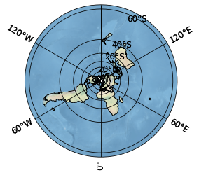
This plot now shows the entire northern hemisphere. We are however only interested in the arctic, so we adapt our lonlatbox
[3]:
sp.update(lonlatbox=[-180, 180, 60, 90],  # lonmin, lonmax, latmin, latmax
          # disable the grid
          xgrid=False, ygrid=False)
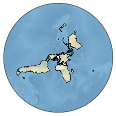
We can also use the clon and clat formatoptions to focus on Greenland. Here, we might also want to change the projection since the northpole projection implies clat=0
[4]:
sp.update(clon='Greenland', clat='Greenland', projection='ortho', lonlatbox=None)
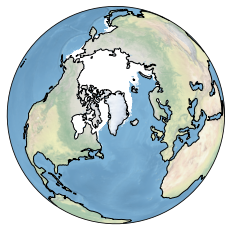
Despite the beautiness of these plots, there are a few things to notice when it comes to circumpolar plots
Usually, psy-maps interpolates the boundaries for 1D-plots (see the
interp_boundsformatoption), which is by default disabled for two-dimensional coordinatesAs stated above, circumpolar grids have two dimensional coordinates. Those coordinates have to be specified in the
coordinatesattribute of the visualized netCDF variable (see the CF Conventions on Alternative Coordinates). It is important here that the dataset has not been opened using thexarray.open_datasetmethod, since this will delete thecoordinatesattribute. Instead, use thepsyplot.project.open_datasetfunction which also interpretes the coordinates but does not modify the variable attributes.Unfortunately, the CF-Conventions do not specify the order of the coordinates. So the coordinate attribute could be ‘longitude latitude’, ‘latitude longitude’, ‘x y’ or ‘y x’ or anything else. This causes troubles for the visualization since we do not know always automatically, what is the x- and what is the y-coordinate (except, the
axisattribute has been specified). If we cannot tell it, we look whether there is alonin the coordinate name and if yes, we assume that this is the x-coordinate. If you want to be 100% sure, create the decoder for the data array by yourself and give the x- and y-names explicitlyfrom psyplot.data import CFDecoder ds = psy.open_dataset('netcdf-file.nc') decoder = CFDecoder(x={'x-coordinate-name'}, y={'y-coordinate-name'}) sp = psy.plot.mapplot(fname, decoder=decoder)
For more information, see the get_x and get_y methods of the CFDecoder class
To sum it all up: 1. by default, circumpolar plots are slightly shifted and the last column and row is not visualized (due to matplotlib) 2. Do not use the xarray.open_dataset method, it will delete the coordinates attribute from the variable 3. Be aware, that a coordinate listed in the coordinates meta attribute that contains a lon in the name is associated with the x-coordinate.
[5]:
psy.close('all')
Note
To highlight the differences between xarray.open_dataset and psyplot.project.open_dataset just look at the Attributes section of the two variables in the variables below
[6]:
import xarray as xr
print('Opened by xarray.open_dataset')
print(xr.open_dataset('G10010_SIBT1850_v1.1._2013-01-15_circumpolar.nc')['seaice_conc'])
print('Opened by psyplot.project.open_dataset')
print(psy.open_dataset('G10010_SIBT1850_v1.1._2013-01-15_circumpolar.nc')['seaice_conc'])
Opened by xarray.open_dataset
<xarray.DataArray 'seaice_conc' (y: 180, x: 180)>
array([[-1., -1., -1., ..., -1., -1., -1.],
       [-1., -1., -1., ..., -1., -1., -1.],
       [-1., -1., -1., ..., -1., -1., -1.],
       ...,
       [-1., -1., -1., ..., -1., -1., -1.],
       [-1., -1., -1., ..., -1., -1., -1.],
       [-1., -1., -1., ..., -1., -1., -1.]], dtype=float32)
Coordinates:
    lon      (y, x) float64 ...
    lat      (y, x) float64 ...
Dimensions without coordinates: y, x
Attributes:
    standard_name:  Sea_Ice_Concentration
    long_name:      Sea_Ice_Concentration
    units:          Percent
    short_name:     concentration
Opened by psyplot.project.open_dataset
<xarray.DataArray 'seaice_conc' (y: 180, x: 180)>
array([[-1., -1., -1., ..., -1., -1., -1.],
       [-1., -1., -1., ..., -1., -1., -1.],
       [-1., -1., -1., ..., -1., -1., -1.],
       ...,
       [-1., -1., -1., ..., -1., -1., -1.],
       [-1., -1., -1., ..., -1., -1., -1.],
       [-1., -1., -1., ..., -1., -1., -1.]], dtype=float32)
Coordinates:
    lon      (y, x) float64 ...
    lat      (y, x) float64 ...
Dimensions without coordinates: y, x
Attributes:
    standard_name:  Sea_Ice_Concentration
    long_name:      Sea_Ice_Concentration
    units:          Percent
    short_name:     concentration
References
CDO 2015: Climate Data Operators. Available at: http://www.mpimet.mpg.de/cdo
Walsh, J. E., W. L. Chapman, and F. Fetterer. 2015. Gridded Monthly Sea Ice Extent and Concentration, 1850 Onward, Version 1. Boulder, Colorado USA. NSIDC: National Snow and Ice Data Center. doi: http://dx.doi.org/10.7265/N5833PZ5. Accessed 26.09.2017.